We use the motivating example of farmers choosing seeds to sow, in order to study how individuals or firms should best respond to large and infrequent negative or positive events. We consider two types of related but fundamentally difffernet problems a farmer may face. First, how much "experimenting" should a farmer do with his or her own land? Secondly, how should a farmer diversify crop planting in order to hedge against the possibility of disease.
When farmers decide what kind of seed to sow, we assume they decide in accordance with their preference for exploration and their preference for diversity. A farmer with a high-exploration prefrence may decide that using land to take a chance on finding a new, high yield and patentable crop, is worth while. A farmer with a low exploration preference will exploit the knowledge he or she already has about seeds and their projected crop yields. A farmer who is unconcerned with diversity will maximize his harvest yield in most cases by planting exclusively the seed that is projected to be the most productive, but will be more vulnerable to a very low yield whenever disease strikes, as the farmers entire crop could be destroyed. Our aim is to explore which farming strategies fare better over time, under a variety of circumstances.
The model contains a community of 10 farmers that each have 10 plots of land. Each farmer will plant one seed on each plot of land. Each farmer is seeking to maximize their profit for any given year, which is defined by the yield of their harvest minus the costs they pay to other farmers for patented crops. Each crop seed is represented by a 10 bit string of 1's and 0's. There is a function, unknown, to the farmer, that assigns a harvest value to the string of 1s and 0s. The function has one parameter for each of the 10 bits that is selected from a uniform distribution from –1 to 1. The value of the crop is the sum product of the bit string with –1's taking the place of 0s, and the string of 10 parameters. Each year, the parameters of this unknown function are changed by a random normal variable with a mean of zero and a standard deviation that we vary from simulation to simulation ("crop drift"). The parameters are not allowed to shift outside of the initial window o –1 to 1.
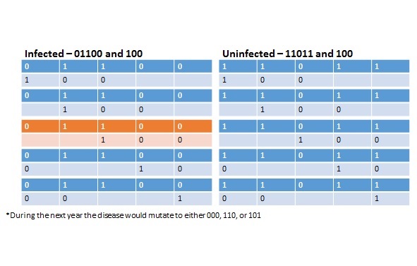
Another parameter that we vary is the frequency of disease in the model. The disease is a string of length defined by the user, if the bit string matches the 10 bit seed string at any point, the diseased crop produces a harvest of zero for that turn. Thus, smaller strings will destroy a larger variety of seed crops. The disease also can "wrap around" the seed string, so if the first 3 bits of a 6 bit disease match the last 3 bits of a seed, and the last 3 bits of the disease match the first 3 bits of a seed, it is considered a match. The probability of a seed being struck by a disease is thus S*2^(D–S)/S^2, where S is seed length and D is disease length. For our models we use a 10–bit seed, and disease lengths of 5, 7, and 9. These give us disease probabilities of 320/1024, 80/1024, and 20/1024 respectively. Each year, one bit mutates (flips from a 1 to a 0 or a 0 to a 1) randomly and has thus the potential to kill a different subset of crops. An example of this process is shown for a 5–bit crop and a 3–bit disease in Figure 1 below:
Each farmer is given a biodiversity preference B, between 0 and 1, and an exploration preference E, also between 0 and 1. These parameters determine how farmers select which seeds to sow in their plots of land. Randomly selected unknown crops are planted on a proportion of their plots equal to E. Farmers also have knowledge of how crops have fared in the past. The remaining ( 1–E) plots are planted with crops where the farmers know how much harvest the crop yielded to the farmer the last time it was planted, or, how much the crop yielded when it was initially patented by another farmer. The farmers plant the crop c in a plot that maximizes perceived utility U, where H is the anticipated harvest and P is the patent cost:
U₂ = H₂ – P₂ – (other plots with crop C ⁄ Total plots)*B
To calculate the actual harvest H for each farmer F, with disease D indicating whether a crop has been wiped out by a disease, we use:
HF = ∑*(1 – DC) – PC
Thus, each farmer is seeking to maximize their harvest, but some have a prefernece for diversity that could protect them from a catastrophically low crop yield if their crop of choice is struck by disease. And some have a preference for the long term potential of patent revenue and/or higher harvest yields from new unexplored crops. Each year, the 2 farmers with the lowest total harvest are removed and replaced by two new farmers. The two new farmers are given parameter values for biodiversity and exploration that are randomly selected from the 4 highest performing farmers, each parameter is chosen independently and a small amount of noise is added to the parameter. This can be thought of as a very simple genetic algorithm. The new farmers knowledge of crops, however, is limited to crops that have been patented.
Initially, a set of 10 farmers is generated with randomly distributed preferences, and knowledge of the performance of only one randomly selected crop that is patented by a farmer outside of the system. (When farmers plant this crop, they incur a patent cost, but no other farmer recieves it). Additioanlly, a crop function is randomly selected, as well as an initial disease. Afterwards, each "year" in the model corresponds to one cycle through all steps, in the following order:
We ran 10 simulations varying across 6 different levels of crop drift (0.01,0.025,0.05,0.1,0.2 and 0.4) and 3 differents levels of disease length (5 bits, 7 bits, and 9 bits), for a total of 180 simulations. We expect that simulations with high levels of crop drift will select farmers who are more willing to dedicate their crops to exploration. We expect that simulations with lower disease length (and thus higher disease frequency) will select farmers who have a higher preference for crop diversity. Each simulation was run for a total of 500 years. An example protohistory is shown below, for one of the simulations with crop drift = 0.05 and disease length = 7 bits:
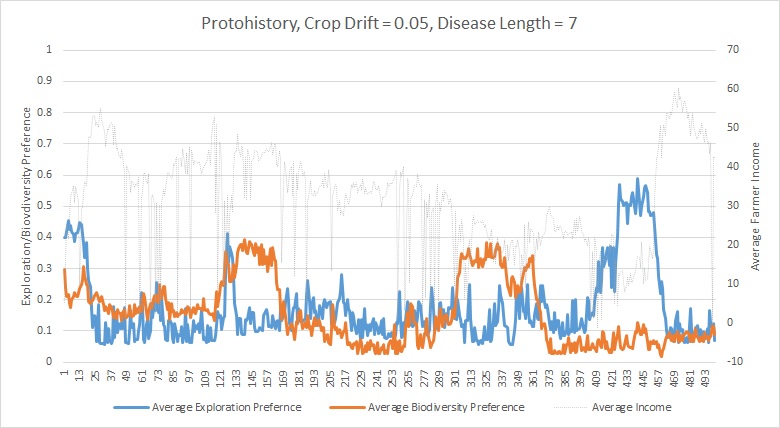
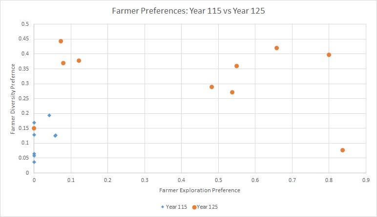
As this protohistory shows, drops in income (presumably from disease) cause the removal of farmers with low exploration and low exploitation values, thus leading to a temporary period of higher biodiversity and/or higher exploration. For example, in years 118 and 122 of this simulation, average farmer income is below 10, although it had previously been around 150. Looking at the distribution of farmer preference in year 115 and 125, we can tell that these shocks caused serious changes:
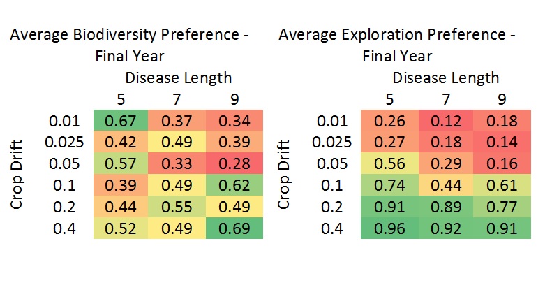
Looking at the 180 simulations in aggregate is difficult, but what we can do is examine the average farmer preferences across all 10 simulations, for each of the 18 different conditions of interest, during the final year of the simulation. Looking at the average preference of farmers for exploration, we see that the preference for exploration increases as a function of disease length decreasing (meaning that disease frequency increases), and as crop drift increases. These results are consistent with what we would expect. Biodiversity preference varies when crop drift levels are higher, however, in these cases if exploration preferences are already high, then preferences for biodiversity are irreleveant (partially as a consequence of model design). When crop drift levels are at their lowest (0.01), diversity does seem to increase as a negative function of disease length. Which is consistent with our expectations. These parameters are all summarized below in Figure 4.
The model we build presents somewhat obvious solutions to two types of problems a farm or another business may face: in a competitive landscape how should individuals balance exploiting the knowledge they have, learning new ways to make profit, and staying robust in the face of unpredictable catastrophic events. As the likelihood of highly negative and highly positive events increases, farms that do not place all their eggs in one basket tend to be the ones that survive.
This model could also help us understand several other issues relevant to both social scientists and policy analysts. For example, nations that have greater levels of cultural, genetic, or ideological diversity may have better long term outcomes. Thus our results could suggest that nations with more favorable attitudes towards immigration are stronger in the long run. Along similar lines, organizations that seek diversity in terms of religion, culture, race, gender, educational background, or other attributes that could correlate with differing ways of thinking, reasoning, or working, may perform better in less predictable market conditions. This presents a potential results driven justification for practices such as affirmative action. Less diverse organizatoins may perform well in stable market conditions, but might not be as robust to external shocks and rare events. At the level of the individual, this model suggests that individuals who are educated in a wide variety of areas are less likely to become obsolete as opportunities for employment shift across different sectors of the economy.
Our overall conclusion is obvious, yet important. Diversity and exploration are not always immediately useful, but they provide necessary security against the unpredictable in the long run.